In the widest sense of the word, the reliability of a system is associated with its correct operation and the absence of breakdowns and failures. However, from the engineering standpoint, this must be quantitatively defined as a probability. Thus reliability is defined as the probability of a system complying with the functions for which it was designed, under certain given specifications and over a determined period of time.
Different types of reliability are defined:
- Specified reliability: the reliability value that the equipment must achieve.
- Inherent reliability: the reliability value resulting from project conception, with no intervention by the degradation that is usually caused when manufacturing the system and its components.
- Estimated or expected reliability: this is the value obtained based on data logs at a specific confidence level.
- Proven reliability: The reliability value obtained by measuring a series of units, with a specific confidence level.
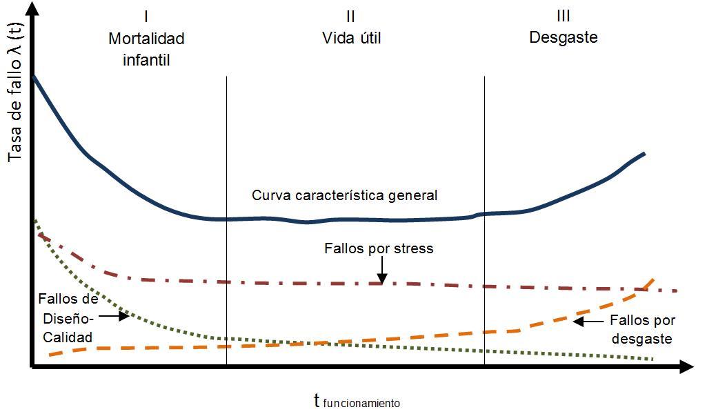
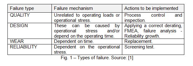
In general, the distribution of the different types of failures (Fig.1) that emerge throughout the lifetime of a specific driver, are combined to give what is known as the "bathtub curve", which traditionally divides the lifetime of a driver into the early infant mortality phase, the useful life phase and the wear out phase.
The failures caused by design and quality defects usually display a marked downwards incline and dominate the infant mortality phase. The useful life phase of mature electronic drivers features a small and constant failure rate, which approximately follows a law of exponential distribution and is governed by the intrinsic defects related to electrical and thermal stresses etc. that randomly occur. Finally, during the wear out phase, failures caused by component fatigue can arise.
The aim of the reliability programme is to guarantee a short infant mortality phase and a long useful life period with a failure rate stabilised at a low level. For this, during the design and development phase and during the subsequent industrialisation, measures have to be taken that evaluate the impact of the intrinsic defects and those induced by the manufacturing process, which guarantee the efficiency of conventional inspections and the effectiveness of the reliability screening tests applied. Specifically, the reliability programme phases are:
- High level design
- Initial reliability prediction
- Reliability allocation
- FMEA
- Thermal analysis
- Tolerance analysis
- Component derating
- Final reliability prediction
- ESS – Environmental Stress Screening
- Demonstration of reliability
INITIAL RELIABILITY PREDICTION
The objective of the reliability prediction is to estimate the failure rate that a driver will have during its useful phase, so that the designer is able to evaluate the capacity of their design to comply with the specified reliability requirement and can identify the design blocks that require the application of a special stress.
Most of the reliability prediction models are founded on empirical databases and are subjected to two sources of variability:
- The estimates used are averages and do not take into account variances or confidence intervals.
- The averages used as estimates are based on products manufactured in the past, meaning that subsequent improvements that have been made to the reliability of the components are not reflected. To solve the problem, the reliability engineer sometimes applies corrective factors that take into account the reliability improvement achieved over time by the maturity of the technologies.
As such, by analysing the expected failure rate for a product and comparing it with others, we can be sure that the reliability prediction model used is the same in both cases and that the same corrective factors have been applied.
In addition, we must not lose sight of the fact that the result of the prediction is the inherent reliability of the driver, which is the outcome of the project conception. It does not take into account defects in the raw materials or the degradation to the reliability that occurs while manufacturing the unit, or that which could arise when installed under conditions different to those expected.
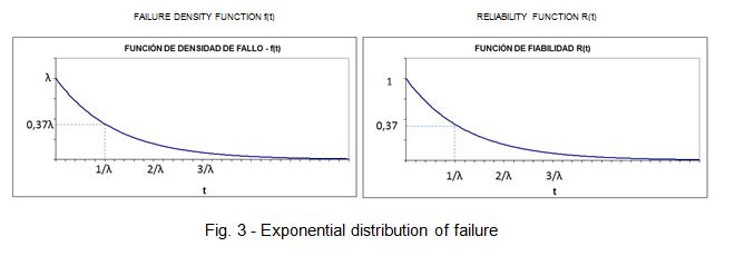
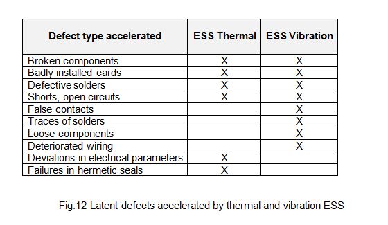
The reliability prediction models assume that the failure probability distribution that follows the electronic drivers and components is exponential, with a constant failure rate λ. As such, they are only valid to estimate reliability during the useful life stage of the bathtub curve, in which the failure rate remains constant. Thus the reliability function or the probability that the driver survives up until a determined moment t will be:

The exponential distribution has two distinct properties that are highly important in reliability:
- “It has no memory”, in other words: the probability of a driver failing at some time in the future is independent to the age of the device.
- The failure rate of drivers in series, is the sum of the failure rates of each one of them.
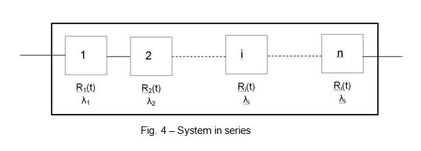
A constant current driver for outdoor LED street lighting, constitutes a system in series because if one component fails, it could be said that the entire system has failed. The probability of survival of a system in series is equal to the outcome of the survival probabilities of each component in series, assuming they operate independently, where the failure rate of the system driver is the sum of the failure rates of all the components it comprises. And for drivers that cannot be repaired, the average time up until the failure is the inverse of the failure rate of the driver.
During this initial development phase of the driver, the reliability prediction takes place using the part count model, as set out in Appendix A of the MIL-HDBK-217F(N2) [2]. In this model, the failure rate of the driver, λsystem, is calculated as described above, but introducing a quality factor πQ, which values the components that comply with the military standards of the United States Department of Defense and whose values range from 0.01 for a component subjected to every screening test specified by those military standards, to 10 for a commercial component. Therefore:
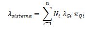
where:
n: number of generic families of components in the product.
λGi: generic failure rate of the ith generic family of components.
πQi: quality factor of the ith generic family of components.
Ni: quantity of components of the ith family present in the product.
The MIL-HDBK-217F(N2) has not been updated since 1995 and therefore does not take into account the improvements in reliability achieved over the past 23 years. As a result it offers a very pessimistic forecast of the failure rate, far removed from the reality demonstrated by use in the field. In addition, it penalises standard commercial components with a multiplier of up to 1,000 times the failure rate. To adjust the prediction more to the reality, it is useful to apply the adjustments contemplated in the ANSI VITA 511.1 standard, which is subsidiary to the MIL-HDBK-217F(N2) [4].
As such, the first step is to define a high level design of the driver the object of the reliability programme. The design team, based on its experience and previous designs, will evaluate the number of components of each one of the generic families: Microcircuits, Discrete Semiconductors, Resistances, Condensers, Inductives and Sundries (terminals, PCB, fuses, etc.) that comprise each block. With this data input into the MIL-HDBK-217 tables, a first prediction is obtained for the failure rate of the λdriver = 1,294 failures per million operating hours, which represents a rate of 0.1294% per 1,000 hours and an MTTF (Mean Time To Failure) of 772,797 hours. This means that the expected reliability for a service life of 100,000 hours is 88%. In other words, 88% of the population would achieve 100,000 hours of useful life, or to put it another way, the probability that a driver survives 100,000 hours is 88%.
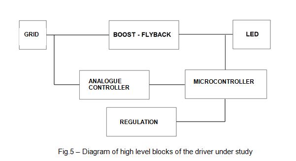
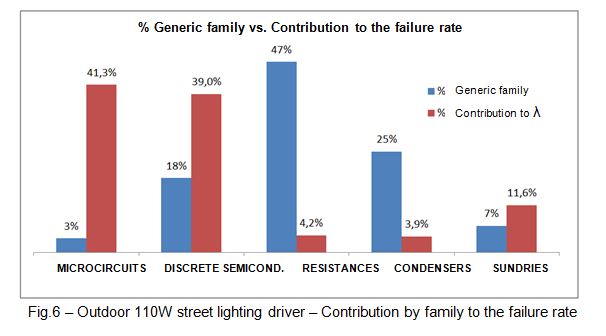
A distribution by generic family of components is also obtained, providing a reference for the design tasks. For example, it can be observed that the generic family of microcircuits (microprocessors, memories, linear microcircuits, etc.) that represents 3% of the expected components, has a contribution to the expected failure rate of 41.3%. As such, an investment in improving their reliability should be weighed up.
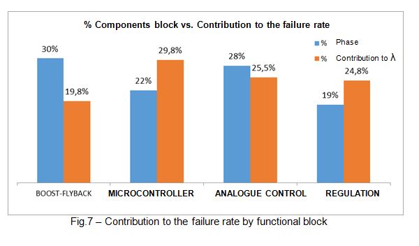
Similarly, the distribution by blocks indicates that there is room for reliability improvement during the design phase, above all in the controller and regulation blocks.
ALLOCATION OF RELIABILITY OBJECTIVES
With the initial forecast data of the failure rate and its distribution by families of components and by functional blocks, an expected reliability objective can be allocated to the driver once designed. And that overall system failure rate is distributed between the various functional blocks of the design. This focuses the development engineers on the critical points on which they must work to achieve the proposed reliability objectives.
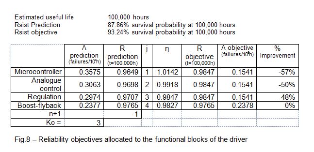
In the case studied, an objective was set of 0.7 failures every 106 hours (MTTF: 1,43x10⁶ hours), or a failure rate of 0.07% per 1,000 hours. As such, the aim is that the probability that a specific unit of the driver continues working once it reaches its estimated useful life of 100,000 hours is R(t) = 93.24%.
There are many options when the time comes to allocate reliability objectives during this initial design phase. They can be equally distributed between every block (equitable technical allocation). Coefficients can be allocated to each block depending on the state-of-the-art, the complexity of each block, ambient conditions, etc. (objectives feasibility technique).
For this case study, the method used to allocate objectives is known as the “effort minimisation algorithm”, that aims to minimise the effort required to achieve the allocated reliability objective. The method assumes that the reliability of each functional block has been predicted and that greater improvements to the blocks with the lower initially expected reliability will be required. Fig. 8 sets out the reliability objectives proposed by the designers for each one of the blocks. The overall improvement proposed was 42% over the initial estimate.
DESIGN TECHNIQUES FOR RELIABILITY
Design techniques for reliability are used to ensure that the reliability objectives are achieved in the final product. For the constant current LED technology driver for outdoor lighting, the object of this study, the following techniques were used:
a. Management of suppliers and components. It is very important that suppliers and components are selected that offer reliability datalogs and carry out screening tests. A high volume and continuous production is recommended, given that the capacity to manufacture defect-free components is directly linked to failures. The reason is that the improvement cycle is shorter, because failures occur earlier and are analysed more frequently, enabling a faster growth in reliability.
b. Derating. This is defined as making a component work subjected to stress that is lower than nominal levels. This can decrease the stress or increase the resistance of the component. It is effective because the failure rate tends to decrease as the stress level applied to the driver reduces. The reliability of the electronic components is a function of the electrical and thermal stresses. A higher thermal stress generally involves a higher bonding temperature which accelerates the chemical activity of the component, as expressed by the Arrhenius model, resulting in a greater failure rate.
c. Analysis of circuit tolerances. With ageing and stress, the values of the physical and electrical parameters of the components tend to experience variations that, if not taken into account during the design, can degrade the performance of the circuit and become a significant cause of failure. They must also take into account the variations in the electrical parameters of the components that originate from variability in the manufacturing process. The designer will aim to achieve the greatest level of system insensitivity to such variations.
d. Failure Mode and Effects Analysis (FMEA) The Design Failure Mode and Effects Analysis is an analytical and systematic technique that evaluates the probability of failure and its effects. It is a proactive tool from which preventive measures against possible failures are obtained.
e. Design for the fabricability and assembly. This is a concurrent engineering process that aims to optimise the relation between the design function, fabricability and the ease of assembly. Thus the introduction of patent and latent defects during the manufacturing of the driver is reduced.
FINAL RELIABILITY PREDICTION – INTRINSIC PREDICTION
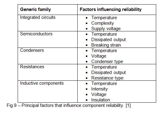
At the end of the design phase, the materials list will be complete and available to the reliability engineer. Having manufactured the first prototypes, the electrical, thermal and mechanical stresses to which the components are subjected are already available. This then enables a more detailed reliability prediction to be calculated. For this, despite having been conceived for military applications and not updated since 1995, this model continues to be the most widely-used in the electronics industry: that corresponding to the component stress analysis or “Part Stress Analysis” developed by the MIL-HDBK-217F(N2). The method associates a basic failure rate with each generic family of components that is modified by multiplying some coefficients that represent the factors affecting reliability (Figure 9):
Thus, for example, for a ceramic condenser, the failure rate is calculated as:
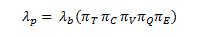
where:
πT : Acceleration factor due to the temperature.
πC : Capacity factor.
πV : Voltage stress factor.
πQ : Quality factor that depends on applicable military standards.
πE : Ambient operating factor (land, sea, air...).
And for a monolithic bipolar device, the intrinsic failure rate is calculated as:
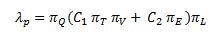
where:
πL : Technological maturity factor of the generic family.
πQ : Quality factor that depends on applicable military standards.
πT : Acceleration factor due to a temperature.
πV : Voltage stress factor.
πE : Ambient operating factor (land, sea, air,...).
C1: Microcircuit complexity factor.
C2: Enclosure complexity factor.
In the case studied, the objective for the LED technology driver for street lighting was set at 0.7 failures for every 106 hours (MTTF: 1.43x10⁶ hours), or a failure rate of 0.07% for every 1,000 hours. Following the design and development process undertaken, taking into account the reliability engineering concepts, the results shown in Fig. 10 were obtained. The objective was improved by 1.3%.
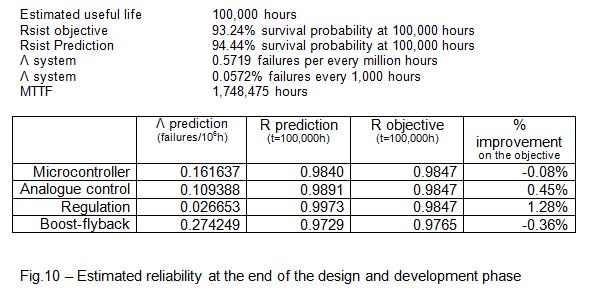
Having obtained the expected reliability figure of an MTTF of 1,748,557 hours (203 years), it is interesting to consider that this should not be thought of as the time that a product is expected to survive once installed. In other words, this is not the estimated useful life, or the expected lifetime in at least 50% of the installed drivers.
The MIL-HDBK-217-F(N2):
- Calculates an intrinsic reliability, which is why it neither takes into account the causes of the failure introduced by the productive process nor those introduced by the installation conditions.
- Does not take into account infant mortality failures or those occuring during the wear out period.
- It is based on the commonly-used premise in the electronics industry that the failure probability distribution during the useful life period follows an exponential law in which the probability of survival up until a specific moment the time is:
In other words, due to the definition of the exponential distribution, the probability that a driver survives up until it acheives its MTTF is 37%. This should not be confused with the useful life of a driver.
ENVIRONMENTAL STRESS SCREENING
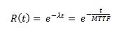
As mentioned above, inherent reliability is a consequence of poducte design. However, without a programme that guarantees reliability during production, the reliability inherent to the product can be severely degraded due to the defects introduced thanks to problems with components or as a result of the manufacturing process. Some are revealed during inspections, but others remain as latent defects until a specific operating condition accelerates that failure.
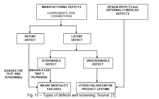
Environmental Stress Screening (ESS) aims to precipitate those latent defects whose failure mechanism can be accelerated. The most commonplace types of ESS are temperature cycles, random vibrations, sinusoidal vibrations, on-off cycles, burn-in cycles at high temperatures, etc. The latent defects that can be accelerated by ESS are set out in the table in Fig. 12.
In our case study, the programme used includes thermal and vibration ESS. The testing conditions followed were similar:
- The drivers were tested before the ESS in order to ensure that no previous patent failures existed.
- The drivers were tested again once the ESS had finished, applying the same tests as before the ESS to determine if any latent defect had been accelerated or not.
- The drivers under ESS were connected and the stress to which they were subjected was representative of normal usage conditions.
- The ESS is defined by its Screening Strength (SS) which is the percentage of latent defects capable of being accelerated by the test.
- The tests described below were developed by the RADC (Rome Air Development Center) using its “Stress Screening of Electronic Hardware" [10] and “Environmental Stress Screening” [11]. These references explain how the SS formulae were calculated that were used in the tests described below.
a. ESS vibration test at a single frequency. The SS is a function of the acceleration level in numbers of “g”. The test took place at 0.03G. It is also a function of the test duration in minutes. It was tested over 10,140 minutes.
The sample tested included 40 units and no defect was accelerated. The calculated SS indicates that 99.07% of latent defects are accelerated. As such, the latent defect level in production that can be accelerated using this method will be less than 0.13%.
b. ESS test at a constant temperature. In this test, the SS depends on the difference between the test temperature and 25ºC, which in this case was 17ºC, as the test took place at a temperature of 42ºC. The test lasted 1,440 hours.
40 units were tested and no defect was accelerated, where the SS should detect 99.999% of latent defects. As such, the latent defect level will be less than 0.001%.
The ESS programme thus provides a reasonable degree of security that the latent defect rate introduced by the components themselves or by the manufacturing process of the driver, is sufficiently small so as to not compromise the reliability objective in the field.
DEMONSTRATION OF RELIABILITY
a. Before launch. The length of the useful life currently demanded from electronic drivers makes the application of the reliability inspection by sampling every lot impractical. This is because the length of the tests required to demonstrate reliability, exceeds commercially reasonable timeframes. However, there is still a need to demonstrate reliability, at least in pre-industrialised series. To do this, the sample tables contained in the MIL-HDBK-108 [12] can be used. For a driver with a useful life of 100,000 hours, a possible plan to demonstrate reliability would be:
- Available duration for the test: 5,000 hours.
- Acceptable average life: 100,000 hours.
- Unacceptable average life: 33,333 hours.
- Manufacturer risk α: 0.10 (if the average life is greater than 100,000 hours, it will be rejected with a probability of 10%).
- Buyer risk: 0.10 (if the average life is lower than 33,333 hours, a probability of 10% will be accepted).
- No. of samples to be tested: 63 units.
- No. rejected: 6 (if less than 6 fail, the pre-series will be accepted, as was the case after 1 recorded failure).
b. Monitoring in the field. Once the driver starts to be commercialised, the data on operating hours and failures recorded in the field must be monitored, providing the reliability engineer with a greater amount of data with which to calculate the confidence interval for the MTTF of the driver under real conditions. The equation for the confidence interval is statistically calculated as a function of the test time, of the level of significance of the test that is aimed to be achieved and the number of failures that occur during the test period.
For our case study, currently, the accumulated operating time of the drivers in the field is T = 1,125,367 hours, having detected 1 failure. As such, at these times, the exceptional estimated MTTF is 1,125,367 hours with a survival probability at 100,000 hours of 92%. The confidence interval for the true value of the MTTF is (234.351, ∞) hours, with a confidence level of 90%.
Frequent monitoring of this interval, along with the comprehensive analysis of the units returned from the field, is able to detect if the reliability level degrades, applying any corrective actions that may be necessary.
CONCLUSIONS
The design and application of a reliable engineering programme is an essential requirement throughout the development process as it increases user satisfaction, guaranteeing high levels of availability and trust in the street lighting drivers and systems. It allows an efficient preventive maintenance strategy to be established and provides a solid basis on which to calculate the offered product guarantees.
Juan José González Uzábal
ELT Quality and Industrial Director